Which Bike Was It? Strava Ride Classification with R

Sep 22, 2019
Every month, Google gives me a summary of how much much I’ve traveled. It’s really cool to look at, but one creepy feature about it is that it gives me a breakdown of how much I’ve traveled by medium. travels

There are even motorcycle riders’ blogs where discussions have taken place about how Google know’s they’ve ridden their motorcycles as opposed to their cars.

One could probably guess that Google is using GPS information from our phones using speed, roads traveled and similar factors to make estimations about how we’re getting around.

I ride bikes a fair bit, and use 2 different bikes to get around. I set out to try something similar. I log my rides on Strava, it gives the athlete the option to choose which bike they rode. I happen to have 2 bikes, one for road riding and the other for gravel riding and cyclocross.

Getting my rides from Strava

Retrieving my rides from Strava involved using their API. Here’s a good post detailing the steps for ‘creating an application’ to allow you to get your data. The API response is in JSON format, but the jsonlite package makes it easy to flatten.

The max number of activities per API request is 200, so i needed to make a couple of requests to get a large number of rides. Combinining the two into a single data frame wasn’t trivial, as the tables had a different number of variables.

token <- Sys.getenv("token")

stuff <- paste0("https://www.strava.com/api/v3/athlete/activities?access_token=",token,"&per_page=200&page=1") %>% fromJSON(flatten = TRUE)

stuff2 <- paste0("https://www.strava.com/api/v3/athlete/activities?access_token=",token,"&per_page=200&page=2") %>% fromJSON(flatten =TRUE)

names1 <- names(stuff) %>% tbl_df()
names2 <- names(stuff2) %>% tbl_df()

names1 %>% anti_join(names2) %>% kable()

value
average_heartrate
max_heartrate

I used to ride with a heart rate monitor; it makes sense that these were the extra attributes from the first response.

rides <- rbind(stuff2,stuff %>% select(-average_heartrate,-max_heartrate)) %>% tbl_df() %>%  
    mutate(year = year(start_date)) %>% filter(type=="Ride",
                                               str_detect(gear_id,"b1985937|b3994483")) %>%
    mutate(gear_id = ifelse(gear_id=="b1985937","Road","Gravel"),
           gear_id = as.factor(gear_id))

Exploring

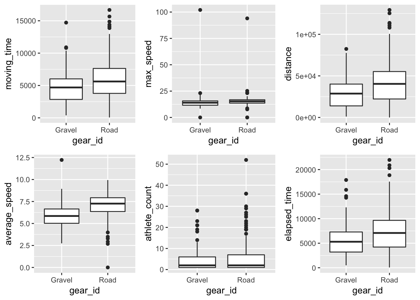
There are a lot of features of a Strava ride. I decided to focus on those that I had the most intuition around: moving time, elapsed time, distance, average speed, athlete count (group rides), and max speed.

library(cowplot)
rides %>% ggplot(aes(y=moving_time,x=gear_id)) + geom_boxplot() ->p1
rides %>% ggplot(aes(y=max_speed,x=gear_id)) + geom_boxplot() -> p2
rides %>% ggplot(aes(y=distance,x=gear_id)) + geom_boxplot() -> p3
rides %>% ggplot(aes(y=average_speed,x=gear_id)) + geom_boxplot() -> p4
rides %>% ggplot(aes(y=athlete_count,x=gear_id)) + geom_boxplot() -> p5
rides %>% ggplot(aes(y=elapsed_time,x=gear_id)) + geom_boxplot() -> p6

plot_grid(p1,p2,p3,p4,p5,p6)

It looked like the most obvious separation comes the difference in average speed between the two bikes.

Building Classification Models

My goal was to come up with a model that classified my 2019 ride data, trained on my 2018 data.

rides_2018 <- rides %>% filter(year==2018)
rides_2019 <- rides %>% filter(year==2019)

Logistic Regression

Starting from a logistic regression model using only average as the only predictor, I tried some different combinations until I landed on one using two interaction variables, one between average speed and distance and the other between average speed and athlete count.

glm_fit <- glm(data=rides_2018, gear_id  ~ average_speed*distance + 
               average_speed*athlete_count,family = "binomial")

contrasts(rides_2018$gear_id)

glm_fitted <- predict(glm_fit,rides_2019,type = "response")

logistic <- data.frame(glm_fitted, rides_2019$gear_id)
logistic <- logistic %>% mutate(glm_fitted = ifelse(glm_fitted<.5,"Gravel","Road")) 

rides_2019 %>% count(gear_id)

mean(logistic$glm_fitted==logistic$rides_2019.gear_id)

## [1] 0.7142857

The logistic model correctly classified 71% of the rides from 2019. This is fair bit better than flipping a coin, but simply guessing that all my rides were road rides would have gotten me results almost as good.

K-Nearest Neighbors

The KNN approach doesn’t bear assumptions about the shape of the decision boundary between road rides and gravel rides. Its flexibility might yield predictions closer to the 2019 data. Here I used the predictor from the logistic model with the lowest p-value, average_speed*distance.

train <- rides$year==2018
test <- rides$year==2019
train_1 <- cbind(rides$average_speed*rides$distance)[train,] %>% as.data.frame()
test_1 <- cbind(rides$average_speed*rides$distance)[test,] %>% as.data.frame()
gear <- rides$gear_id[train] 

set.seed(100)

tests <- for (i in 1:30) {
    oof <- knn(train_1,test_1,gear,k=i)
    ouch <- data.frame(oof,rides_2019$gear_id) ##Choosing the best K for 2019 data
    oops <- mean(ouch$oof==ouch$rides_2019.gear_id)
    print(oops)
}

knn_pred <- knn(train_1,test_1,gear,k=11) 

mean(knn_pred==rides_2019$gear_id)

## [1] 0.7698413

The KNN with a K of 11 produced the model for the 2019 data, accurately predicting the bike I rode for 77% of the data.

Conclusion

These models both show that there is a predictable difference between gravel rides and road rides. Being able to select the bike you rode is a useful feature, but I find it often goes neglected. Perhaps Strava could employ a (much) better model (with an actual method to the subset selection) to choose the best default for the rider depending on their ride data.

In part 2, I’ll use the map coordinates to try and improve these predictions.